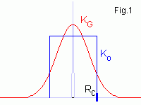
Vi = ∑j= -Rc,Rc fi+j

|
In the applet below you see 1D realisation of white and correlated noise
with equidistant step in x. Independent random points
fi with
uniform distribution on interval (-1, 1) make the white noise (the blue
curve). Correlated random points Vi (the red curve) are
obtained by averaging of white noise in radius Rc sphere, i.e.
kernel Ko is used
Vi = ∑j= -Rc,Rc fi+j |

To get a 2D fractal noise (mountain) you take an elastic string (see Fig.1), then a random vertical displacement is applied to its middle point. The process is repeated recursively to the middle point of every new segment. The random displacement decreases m times each iteration (usually m = 2 are used).

|
Using Fourier transformation for V(r), K(r), f(r)
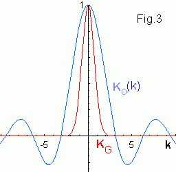
g(k) = ∫ g(r) eikr dr , we get for V(k) V(k) = K(k) f(k) . I.e. averaging (*) means the white noise filtration by means of a filter with bandwidth K(k). The bandwidths for the two used filters are shown in Fig.3 (for Rc = 1) KG(k) ~ exp[-(Rck)2], Ko ~ sin(Rck)/k. |
At last 2D correlated random landscape. To get a smooth potential
2D Gauss kernel is used
Percolation in random potential landscape
Drag mouse to rotate 3D image (with "shift" to zoom it).
The white line (in the blue bar to the right) corresponds to the average
<V> value. The yellow line corresponds to the Fermi energy
εF . Drag the line by mouse
to change εF .
See also 3D Mountains and
Hidden Surface Removal Algorithms.