Ferromagnetic phase transition

By means of the applet below (it uses the Metropolis algorithm) you can make sure that at low temperature (e.g. at T = 1) in equilibrium the system tries to lower its energy and goes to the ordered states with non-zero magnetization M. At high temperature (T >> J = 1) the system goes to the phase space region with high entropy (and disorder). In this case spins orientation is not ordered and magnetization is zero. I.e. there are two phases: ordered with non-zero magnetization and dis-ordered with M = 0. Magnetization determines spins ordering and is called order parameter.
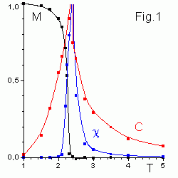
transition It is amazing, that in the 2D Ising model transition between these two phases is remarkably sharp, since M approches zero at critical temperature Tc = 2.2692... with infinite slope. This phenomenon is called the second order phase transition. In this transition order parameter M is continuous but susceptibility χ and specific heat C, which are expressed as the second derivatives of the partition function Z, diverge at Tc . Order parameter is expressed as the first derivative of Z and it is discontinuos at the critical temperature in the first order phase transition.
To observe the phase transition you should change in steps temperature around the critical point. Results of this modelling for 400x400 lattice are shown in Fig.1. Averaging was performed over 400 passes. As it was discussed before, at T = 2.4 relaxation time τr ~ 190, therefore relaxation at the temperature may take place after up to several thousands of passes.

Controls Click mouse to get a new spins configuration. Press "Enter" to set a new T value. You see magnetization M (the red curve) and energy E (the blue curve) in the right part of the applet and in the Status bar. "Print" button sends averaged T, M, χ, E and C to the Java console. "Clear" cleans averaging. See also 640x640 applet window.

Critical exponents for 2D Ising model

Critical exponents for the 2D Ising model are
   M(T) ~ (Tc-T)β,     C(T) ~ |T-Tc|,     χ(T) ~ |T-Tc|,     ξ(T) ~ |T-Tc|,
where β = 1/8, γ = 7/4, ν = 1.
In many cases these exponents are universal, i.e. they do not depend on details of the model, but only on gross features such as the dimention of the space. This explains the success of very simple spin models like Ising model in providing a quantitative description of real magnets.

H.Eugene Stanley "Scaling, universality, and renormalization" Rev.Mod.Phys. 71, S359 (1999).
D.P.Landau "Finite-size behavior of the Ising square lattice" Phys.Rev.B 13, 2997 (1976).


Contents     Previous: Relaxation time     Next: Antiferromagnetics
updated 6 Jan 2002