Bezier spline curves
Linear Bezier spline
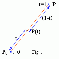
Linear Bezier spline is obtained by linear interpolation between
two control points P0 , P1
P(t) = (1-t)P0 +
tP1 , 0 ≤ t ≤ 1

Interactive Bezier spline
Use finger or mouse to move nearest control point (a small blue square).
In the right window you see basis polynomials of the linear Bezier spline.
The red line is (1-t) and the green one is t.
Images are fitted to your browser window
(sorry if your browser doesn't support HTML5).
Quadratic Bezier spline
Quadratic Bezier spline is obtained by deCasteljau algorithm as
a linear interpolation between linear interpolation between control points
P0 , P1 , P2
P01 =
(1-t)P0 + tP1 ,
P11 =
(1-t)P1 + tP2 ,
P(t) = (1-t)P01 +
tP11 =
(1-t)[(1-t)P0 + tP1 ] +
t[(1-t)P1 + tP2 ] =
(1-t)2P0 +
2(1-t)tP1 + t2P2 ,
P(t) = ∑i=0,2
Bi2(t) Pi ,
Bin(t) = Cni
ti(1-t)n-i ,
Cni = n! / i!(n-i)!
where Bin(t) are Bernstein polynomials.
To the right you see basis polynomials B02(t) ,
B12(t) , B22(t) in the red,
green, blue, ... order.

By construction Bezier spline goes through its terminal control points
(P0 , P2 here)
and is tangent to the first and last segments of the control polygon.
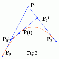
Note that P(t) subdivides the curve in two quadratic splines
(see Fig.2). The new curves match the original in position, although they
differ in parameterization. Points
P0 , P01 , P(t)
and P(t) , P11 , P1
are control points of the new small splines .
Cubic Bezier spline
In a similar way one can use deCasteljau algorithm to
interpolate a curve between (n+1) control points
P0 , P1 ... Pn .
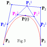
E.g. for n = 3 we get cubic Bezier spline

Points P0 , P01 ,
P02 , P(t)
and P(t) , P12 ,
P21 , P3
are control points of new small splines again.
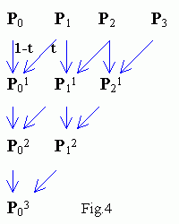
The control points of the two new curves appear along the sides of
the systolic array (see Fig.4 below).
How to plot Bezier spline
DeCasteljau iterations
Pij =
(1-t)Pij-1 + tPi+1j-1,
j = 1, n i = 0, n-j
for n = 3 are shown on the scheme in Fig.4


This algorithm is programmed as (see
bezier.js too)
   for (j = N-1; j > 0; j--)
    for (i = 0; i < j; i++){
      Px[i] = (1-t)*Px[i] + t*Px[i+1];
      Py[i] = (1-t)*Py[i] + t*Py[i+1];
    }
where N = n+1 is number of control points.
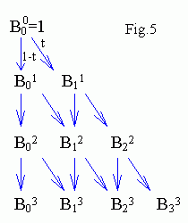
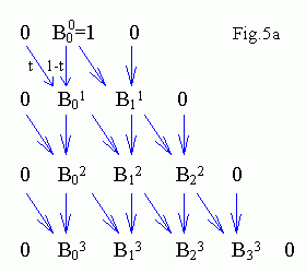
To obtain basis polynomials recurrence relations can be used
B00(t) = 1,
Bin(t) =
(1-t)Bin-1(t) + tBi-1n-1(t),
where Brs = 0 when r < 0 or
r > s.
This algorithm is shown on Fig.5a . It is programmed as
   B[1] = 1;
   for (j = 1; j < N; j++)
    for (i = j+1; i > 0; i--)
      B[i] = (1-t)*B[i] + t*B[i-1];
here B[0] = 0 is added for convenience, therefore i -> i+1.
Basis functions can be obtained too without "zeros" (see Fig.5)
   B[0] = 1;
   for (j = 0; j < n; j++)
    for (i = j; i => 0; i--){
      B[i+1] += t*B[i];
      B[i] = (1-t)*B[i];
    }
Bezier spline of degree n = 7
The general expression for the Bezier spline of degree n
(order n+1) is
P(t) = ∑i=0,n
Bin(t) Pi .
Further you can read More Bezier splines Math or
go directly to Interpolating Lagrange curve.
Contents
Next: More Bezier splines Math
updated 7 August 2001
